Path Loss, Link Budget & System Operating Margins
Path and Free-Space Loss
There are many factors that affect the acceptable maximum range of your Wireless Network with the main culprit being the Path Loss of your wireless signal. Path Loss is a culmination of other factors relating to the signal that include free-space loss, wave refraction, diffraction and reflection, aperture-medium coupling loss and absorption but is also influenced by factors such as geographical contours, the local, natural environment (i.e. foliage) and the propagation medium (i.e. air humidity levels).
Path Loss (attenuation of signal path) is the drop in the density of power (attenuation) of the wireless transmission's wave as it propagates (travels) through a medium over a distance. It is an important element when it comes to the design and planning of a Wireless Network and is a key factor when calculating the link budget.
The Path Loss due to Free-Space Loss will probably be the most important factor when planning Outdoor, long range links with the signal strength being reduced by 4 times if the distance between devices is doubled. Free-Space Loss does not include factors such as the gain of the antennas used at the transmitter and receiver, nor any loss associated with hardware imperfections; it is solely based on the LoS (Line of Sight) path through free space air.
Free-Space Loss can be calculated using the following equations:

Where,
 Free-Space Loss
 Signal’s wavelength (m)
 Distance between transmitter and receiver (m)
Through some further derivation, the following, more practical equation can be used to show the Free-Space Loss in dB (decibels):

Where,
 Free-Space Loss (dB)
Distance between transmitter and receiver (km)
 Signal's frequency (GHz)
Example 1:
If calculating the Free-Space Loss of a 2.4GHz signal, on Channel 6 (2.437GHz) over a distance of 250m:

Example 2:
If calculating the Free-Space Loss of a 70GHz signal (72,000MHz) over a distance of 250m:

You can see from the two examples above, as the frequency increases, the Free-Space Loss (reduction in signal power) increases with regard to distance.
Link Budget
For Wireless Networking connections a Link Budget can be calculated that takes into account all of the gains and losses throughout the link, from the transmitter, to the air and then through the receiver. It looks at signal propagation, antenna gains and other losses from factors such as terrain effects and humidity etc.
A very simplified version of the Link Budget equation can be written as follows:

These simple areas can be broken further into smaller effect variables giving a more practical equation:

Where,
PRX = Received Power (dBm)
PTX = Transmitter Power Output (dBm)
GTX = Transmitter Antenna Gain (dBi)
LTX = Losses from Transmitter (cable, connectors etc.) (dB)
LFS = Free-Space Loss (dB)... this is covered in the chapter above.
LM = Misc. Losses (fade margin, polarization misalignment etc.) (dB)
GRX = Receiver Antenna Gain (dBi)
LRX = Losses from Receiver (cable, connectors etc.) (dB)
In office environments, it is said that LoS propagation only accounts for the first 3m, beyond that indoor losses can increase at up to 30dB per 30m.
Example 3:
If calculating the Link Budget of two identical transceivers operating on a 5GHz signal (5765MHz) over a distance of 500m with transmitter output powers of 21dBm, antenna gains of 14.6dBi, device losses (cable, connecters etc.) of 1.2dB, miscellaneous losses of 0dB and a path loss of 101.5dB:

From this your receiver would have to have a receive sensitivity of -53.7dBm or lower (higher negative value) for your link to operate at all.
System Operating Margin
SOM (System Operating Margin) is a way of calculating the difference between the signal strength the receiver’s radio is actually receiving as opposed to what it actually needs for good data recovery. This is calculated by subtracting the receiver sensitivity value (dB) from the Link Budget figure that was explained in the chapter above.

Where,
SOM = System Operating Margin (dBm)
PRX = Received Power (dBm)
SRX = Receiver Sensitivity (dBm)
For optimum operation, a System Operating Margin of 20dBM or more would be ideal however these values are not always achievable but a value lower than 10dBm is usually considered unacceptable. Shown below is a table showing the relationship between SOM and Availability. 20dBm accounts for a downtime of around 70 hours per year.
SOM (dBm) |
Availability % |
Downtime (per year) |
| 8 |
90 |
876 hours |
| 18 |
99 |
88 hours |
| 28 |
99.9 |
8.8 hours |
| 38 |
99.99 |
53 mins |
| 48 |
99.999 |
5.3 mins |
| 58 |
99.9999 |
32 secs |
Continuing Example 3:
If the Link Budget was calculated to have a received power of -53.7dBm and the receiving device has a receiver sensitivity of -75dbM:

As you can see, the system has an operating margin of 21.3dBm which relates to around 99.4% availability or 2 days 4 hours 42 minutes and 15 seconds of downtime per year.
Maximum Permissible Wireless Network Ranges
If you specify a desired availability for your Wireless Network and the equipment that you want to use, the maximum distance between devices can be calculated by reverse engineering the equations discussed above.
Example 4:
Point-to-Point Wireless Bridge requirements:
- 99.9% availability per year (28dBm)
- 2 identical transceivers operating at 5GHz Channel 36 (5180MHz)
- Output powers reduced to 9dBm for high gain antennas
- Receiver Sensitivity of -67dBm
- Losses in each Transceiver system of 1.2dB
- 2ft Dish Antenna 28dBi Gain

 dB
dB


So you can see, if you have the product characteristics and specified availability, the maximum distance between devices for a specified level of availability can be calculated.
Rain Fade
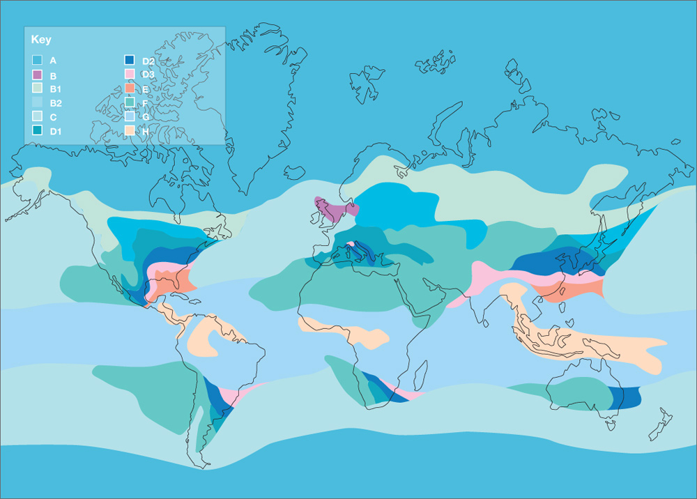
Rain Fade is caused by rain droplets whose separation distance is similar to the signal wavelength and this causes and interruption of communication. This phenomenon has a greater effect on signals above 10GHz where large degradations in signal strength can be caused by heavy downpours or blizzards. A model displaying regional rainfall rates known as the 'Crane Model' can be used to calculate Rain Fade.
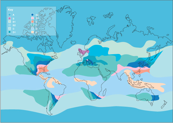
From the diagram above, you locate your Wireless Networking Link location and relate the area to a value which corresponds to certain rainfall rate figures.
Rainfall Rate (R) |
| Percentage of Year (%) |
Region |
A
(mm/hr) |
B
(mm/hr) |
B1
(mm/hr) |
B2
(mm/hr) |
C
(mm/hr) |
D1
(mm/hr) |
D2
(mm/hr) |
D3
(mm/hr) |
E
(mm/hr) |
F
(mm/hr) |
G
(mm/hr) |
H
(mm/hr) |
| 1 |
0.2 |
1.2 |
0.8 |
1.4 |
1.8 |
2.2 |
3.0 |
4.6 |
7.0 |
0.6 |
8.4 |
12.4 |
| 0.5 |
0.5 |
2.0 |
1.5 |
2.4 |
2.9 |
3.8 |
5.3 |
8.2 |
12.6 |
1.4 |
13.2 |
22.6 |
| 0.1 |
2.5 |
5.7 |
4.5 |
6.8 |
7.7 |
10.3 |
15.1 |
22.4 |
36.2 |
5.3 |
31.3 |
66.5 |
| 0.05 |
4.0 |
8.6 |
6.8 |
10.3 |
11.5 |
15.3 |
22.2 |
31.6 |
50.4 |
8.5 |
43.8 |
97.2 |
| 0.01 |
9.9 |
21.1 |
16.1 |
25.8 |
29.5 |
36.2 |
46.8 |
61.6 |
91.5 |
22.2 |
90.2 |
209.3 |
| 0.005 |
13.8 |
29.2 |
22.3 |
35.7 |
41.4 |
49.2 |
62.1 |
78.7 |
112.0 |
31.9 |
118.0 |
283.4 |
| 0.001 |
28.1 |
52.1 |
42.6 |
63.8 |
71.6 |
86.6 |
114.1 |
133.2 |
176.0 |
70.7 |
197.0 |
542.6 |
Also known as Rainfall Propagation, Rain Fade can be calculated using the following equation:

Where,
 Loss in signal strength due to rain (dB)
 Specific attenuation factor due to rain (db/km)
 Network path length (km)
To determine the specific rainfall attenuation value, you must identify some factors depending on your location, availability required and frequency. The equation to calculate this is as follows:

Where,
 Various frequency coefficients
 Rainfall rate depending on availability required in specific region
The Rainfall Rate Value (R) can be taken from the table that was listed above i.e. the R value for a 99.99% available link in region C would be 29.5mm/hr.
k and α can be determined from the table below for either the Horizontal or Vertical polarisation of your devices.
| Frequency (GHz) |
kH |
kV |
αH |
αV |
| 30 |
0.187 |
0.167 |
1.02 |
1.00 |
| 40 |
0.350 |
0.310 |
0.94 |
0.93 |
| 50 |
0.536 |
0.479 |
0.87 |
0.87 |
| 60 |
0.707 |
0.642 |
0.83 |
0.82 |
| 70 |
0.851 |
0.784 |
0.79 |
0.79 |
| 80 |
0.975 |
0.906 |
0.77 |
0.77 |
| 90 |
1.060 |
0.999 |
0.75 |
0.75 |
| 100 |
1.120 |
1.060 |
0.74 |
0.74 |
Example 5:
If a vertically polarised, 80GHz link located in South-West England was required to have 99.99% availability over a distance of 4km, what would the loss in signal strength per kilometre due to rain be?

k = 0.906
South-West England is in Region C so:


So over the 4km link distance, there is 49.08dB lost in signal strength for an 80GHz link at 99.99% availability in that region.